Image Classification with TF 2
Unlike previous versions, TensorFlow 2.0 is coming out with some major changes. It is going to be more pythonic and no need to turn on eager execution explicitly. With tight integration of Keras now it will focus on simplicity and ease of use.
Keras is a high-level API that allows to easily build, train, evaluate and execute all sorts of neural networks. Keras was developed by François Chollet and open-sourced in March 2015. With its simplicity and easy-to-use feature, it gained popularity very quickly. Tensorflow comes with its own implementation of Keras with some TF specific features. > Keras can run on top of MXNet, CNTK or Theano.
![]()
Building a simple image classifier
We will create a simple Neural Networks architecture for image classification. Fashion MNIST is a collection of 70,000 grayscale images of 28x28 pixel each, with 10 classes of different clothing items. We will train our Neural Network on this dataset. > CNN performs better than Dense NN for image classification both in terms of time and accuracy. I have used Dense NN architecture here for demonstration.
Check this article to learn about Convolutional Neural Networks.
Import libraries and download F-MNIST dataset.
import tensorflow as tf
from tensorflow import keras  *# tensorflow implementation of keras*
import matplotlib.pyplot as plt
Download dataset with Keras utility function*
fashion_mnist = keras.datasets.fashion_mnist
(X_train_full, y_train_full), (X_test, y_test) = fashion_mnist.load_data()

print(X_train_full.shape)
(60000, 28, 28)It is always a good practice to split the dataset into training, validation and test set. Since we already have our test set so let’s create a validation set. We can scale the pixel intensities of the data to the 0–1 range by dividing 255.0. Scaling leads to better gradient update.
X_valid, X_train = X_train_full[:5000] / 255.0, X_train_full[5000:] / 255.0

y_valid, y_train = y_train_full[:5000], y_train_full[5000:]
We can view any photo using matplotlib.
plt.imshow(X_train[5])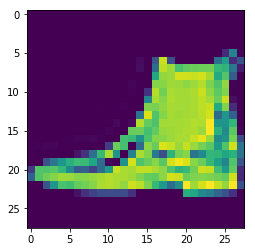
Create a model using Keras Sequential API
Now it’s the time to build our simple image classification Artificial Neural Networks.
model = keras.models.Sequential()
model.add(keras.layers.Flatten(input_shape=[28, 28]))
model.add(keras.layers.Dense(300, activation="relu"))
model.add(keras.layers.Dense(100, activation="relu"))
model.add(keras.layers.Dense(10, activation="softmax"))
If you didn’t get it then don’t worry, let me explain the code line by line.
The Sequential model is a linear stack of layers, connected sequentially.
The next layer, i.e. Flatten is just converting the 28x28 dimension array into a 1D array. If it receives input data X, then it computes X.reshape(-1, 1). It takes an input_shape argument to specify the size of the input data. However, input_shape can be automatically detected by Keras.
The** Dense **layer is the fully-connected neurons in the neural networks. Here, there are two hidden layers with 300 neurons in first and 100 neurons in the second hidden layer respectively.
The last Dense layer made up of 10 neurons in the output layer. It is responsible for calculating loss and predictions.
Compiling the model
Keras has a compile() method which specifies loss function to use, optimizer, and metrics.
model.compile(loss=keras.losses.sparse_categorical_crossentropy,
optimizer="sgd", metrics=["accuracy"])
Train and Evaluate
After the model compilation, we can all fit() method by specifying the epochs, batch size, etc.
Training model
history = model.fit(X_train, y_train,
epochs=30, validation_data=(X_valid, y_valid*))*
This method will train the model for 30 epochs. Train loss, Validation loss and train accuracy, validation accuracy can be found in history.history.
Loss visualization
We can create a visualization for the learning curve using history.
import pandas as pd
pd.DataFrame(history.history).plot(figsize=(8, 5))
plt.grid(True)
plt.gca().set_ylim(0, 1) *# set the vertical range to [0-1]*
plt.show()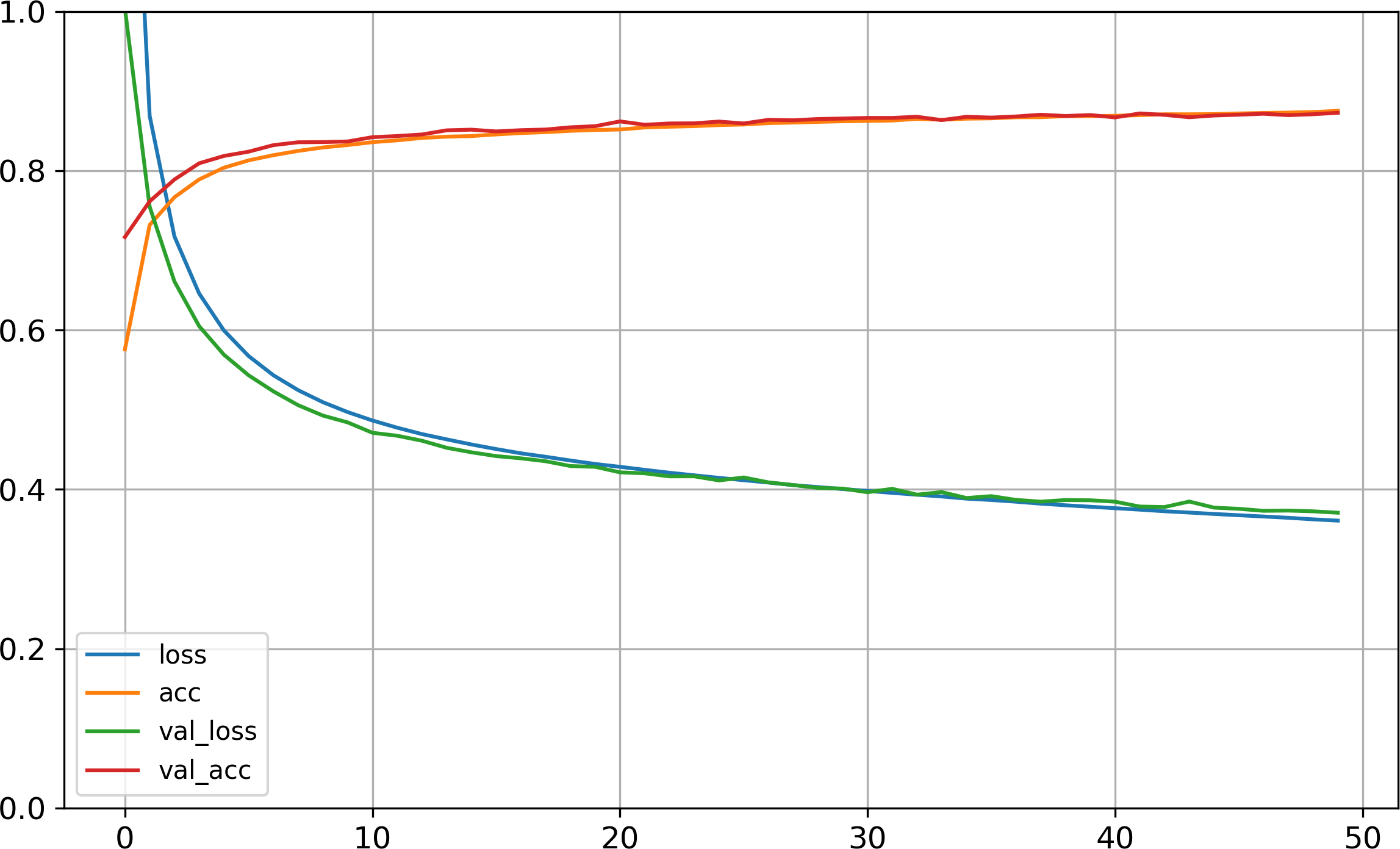 Source: “Hands-on Machine Learning with Scikit-Learn, Keras, and TensorFlow”
We can see that the space between validation and training curves are small that’s why there isn’t overfitting problem.
Now, we can try out different hyperparameters to achieve more accuracy on the dataset.
Model Evaluation
If you are satisfied with the training and validation accuracy then evaluate it on the test set.
model.evaluate(X_test, Y_test)Accuracy on test set might be lower than on validation set because the hyperparameters are tuned for validation set.
Save the trained Model
After you have trained and evaluated your NN model on test set you can download your model using Keras tf.keras.models.save_model method and then can load it anytime for inference.
tf.keras.models.save_model("my_image_classifier")It saves both the model’s architecture and the value of all the model parameters for every layer (All trained weights and biases). This saved_model can be loaded to TF serving for deployment purpose.
If you want to use your trained model for inference, just load it:
model = tf.keras.models.load_model("my_image_classifier")Now, it’s time to train different datasets on your own. Good Luck 😄!
Recommended Resources
Deep learning specialization (Coursera)
“Hands-On Machine Learning with Scikit-Learn and TensorFlow” by Aurélien Géron (Book from O’Reilly)
You can contact me at twitter.com/aniketmaurya or drop an 📧 at aniketmaurya@outlook.com